DQD Search
Stanza provides automated Double Quantum Dot (DQD) search routines for efficiently discovering voltage regions where two quantum dots form with stable charge configurations. After completing health check, DQD search is the next critical step in quantum dot tuning [2], using machine learning classifiers and adaptive grid search to locate promising operating points.
Overview
DQD Search automatically explores the plunger voltage space to find regions exhibiting characteristic double quantum dot charge stability diagrams. The routine follows a systematic multi-stage workflow:
- Peak Spacing Computation - Determine characteristic voltage spacing of Coulomb peaks by analyzing random sweeps
- Grid Generation - Partition plunger voltage space into grid squares based on peak spacing
- Adaptive Grid Search - Use machine learning classifiers to efficiently explore the grid with a three-stage hierarchy
- Intelligent Square Selection - Prioritize regions near confirmed DQDs based on spatial clustering
Each stage builds on previous results, efficiently focusing measurement effort on promising voltage regions while avoiding exhaustive grid scanning.
Prerequisites
Before running DQD search, you must complete device health check. DQD search requires:
- Leakage test results: Safe voltage bounds for sweeps
- Global accumulation results: Global turn-on voltage for gate initialization
- Gate characterization results: Individual gate transition and saturation voltages
See the Health Check documentation for completing these prerequisite routines.
Quick Start
Configure the DQD search routine in your device YAML file:
Then run the DQD discovery sequence:
DQD Search Routines
1. Peak Spacing Computation
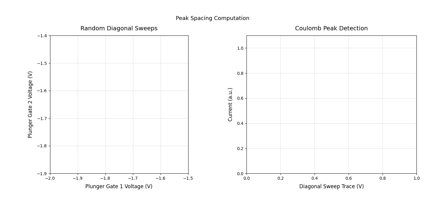
Purpose: Determine the characteristic voltage spacing of Coulomb peaks [3] by analyzing random sweeps through plunger voltage space.
Peak spacing computation provides the fundamental length scale for DQD search by measuring typical distances between charge transitions. This spacing is used to size the grid squares for efficient exploration.
Parameters:
gates(list): All gate electrode names (plungers, barriers, reservoirs)measure_electrode(str): Electrode to measure current from (e.g., “DRAIN”)min_search_scale(float): Minimum voltage scale to test in volts. Typical: 0.05 V (50 mV)max_search_scale(float): Maximum voltage scale to test in volts. Typical: 0.2 V (200 mV)current_trace_points(int, default=128): Number of voltage points per sweep tracemax_number_of_samples(int, default=30): Maximum sweep attempts per voltage scalenumber_of_samples_for_scale_computation(int, default=10): Target number of successful peak detectionsseed(int, default=42): Random seed for reproducibilitysession(LoggerSession, optional): Session for logging measurementsbarrier_voltages(dict, optional): Custom barrier voltages (overrides health check values)
Returns:
peak_spacing(float): Median peak spacing in volts
How It Works:
- Tests multiple voltage scales linearly spaced from
min_search_scaletomax_search_scale - For each scale, generates random diagonal sweeps through plunger voltage space
- Measures current along each sweep and classifies for Coulomb blockade using ML model
coulomb-blockade-classifier-v3 - If blockade detected, uses peak detector (
coulomb-blockade-peak-detector-v2) to identify individual Coulomb peaks - Computes inter-peak voltage spacings and collects statistics across all successful measurements
- Returns median spacing, which determines grid square size:
grid_square_size = peak_spacing × 3/√2 ≈ 2.12 × peak_spacing. This factor ensures the grid square spans approximately three Coulomb peaks along each plunger axis, assuming equal contributions from both gates to the diagonal spacing.
Usage Notes:
- Requires voltage bounds from leakage test (
max_safe_voltage_bound,min_safe_voltage_bound) - Uses gate characterization voltages (transition and saturation) from health check
- Automatically sets plunger voltage bounds based on gate characterization
- Early exits when enough samples collected across all scales
- Raises
ValueErrorif no valid peak spacings detected
2. DQD Search with Fixed Barriers
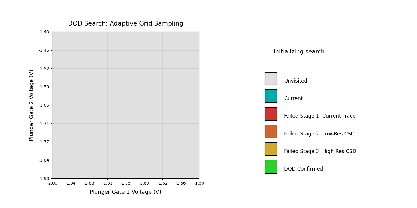
Purpose: Efficiently explore plunger voltage space to find DQD regions using adaptive grid search with a three-stage classification hierarchy.
This routine implements the core DQD search algorithm, using intelligent square selection and multi-resolution measurements to minimize total measurement time while maximizing DQD discovery probability.
Parameters:
gates(list): All gate electrode namesmeasure_electrode(str): Electrode to measure current fromcurrent_trace_points(int, default=128): Points in diagonal current trace for Stage 1low_res_csd_points(int, default=16): Points per axis in low-resolution CSD for Stage 2high_res_csd_points(int, default=48): Points per axis in high-resolution CSD for Stage 3max_samples(int, optional): Maximum grid squares to sample. Default: 50% of total grid squaresnum_dqds_for_exit(int, default=1): Exit after finding this many DQDsinclude_diagonals(bool, default=False): Use 8-connected neighborhoods (True) vs 4-connected (False)seed(int, default=42): Random seed for reproducibilitysession(LoggerSession, optional): Session for logging measurementsbarrier_voltages(dict, optional): Custom barrier voltages
Returns:
dqd_squares(list): List of confirmed DQD squares, sorted by descending total score. Each square contains:grid_idx(int): Linear index in gridcurrent_trace_currents(array): Stage 1 current measurementscurrent_trace_voltages(array): Stage 1 voltage coordinatescurrent_trace_score(float): Stage 1 ML classification scorecurrent_trace_classification(bool): Stage 1 classification resultlow_res_csd_currents(array or None): Stage 2 current gridlow_res_csd_voltages(array or None): Stage 2 voltage coordinateslow_res_csd_score(float): Stage 2 ML classification scorelow_res_csd_classification(bool): Stage 2 classification resulthigh_res_csd_currents(array or None): Stage 3 current gridhigh_res_csd_voltages(array or None): Stage 3 voltage coordinateshigh_res_csd_score(float): Stage 3 ML classification scorehigh_res_csd_classification(bool): Stage 3 classification resulttotal_score(float): Sum of all stage scoresis_dqd(bool): True if high-res CSD classified as DQD
How It Works:
The routine uses a hierarchical three-stage classification to efficiently filter grid squares:
Stage 1: Current Trace (Fast Screening)
- Measures diagonal sweep through grid square (typically 128 points)
- ML classifier:
coulomb-blockade-classifier-v3 - If classification fails, skip to next square (saves 256-2,304 measurements)
Stage 2: Low-Resolution CSD (Intermediate Check)
- 2D grid sweep (typically 16x16 = 256 points)
- ML classifier:
charge-stability-diagram-binary-classifier-v2-16x16 - Confirms DQD-like features with reasonable measurement cost
- If classification fails, skip to next square (saves 2,048 measurements for 48x48)
Stage 3: High-Resolution CSD (Confirmation)
- 2D grid sweep (typically 48x48 = 2,304 points)
- ML classifier:
charge-stability-diagram-binary-classifier-v1-48x48 - High-quality CSD for detailed characterization
- If classification succeeds, square confirmed as DQD
Intelligent Square Selection: After the first random square, prioritizes exploration using spatial clustering:
- DQD Neighbors: Explore unvisited neighbors of confirmed DQD squares (weighted by proximity and scores)
- High-Score Neighbors: Explore neighbors of squares with
total_score > 1.5(passed Stage 1 and possibly Stage 2) - Random Exploration: When no promising neighbors, randomly sample unvisited squares
The search terminates when:
num_dqds_for_exitDQDs are found, ORmax_samplessquares are visited, OR- All grid squares are visited
Usage Notes:
- Requires
peak_spacingfrom priorcompute_peak_spacingroutine - Uses voltage bounds and gate characterization from health check
- Measurements automatically logged if session provided
- Grid squares that exceed voltage bounds are automatically skipped
- Results sorted by descending
total_scorefor easy access to best candidates
3. DQD Search with Barrier Sweep
Purpose: Comprehensive DQD search that sweeps barrier voltages to explore different tunnel coupling regimes.
This routine extends the fixed-barrier search by systematically varying barrier voltages to find optimal configurations. It’s useful when fixed barriers don’t yield DQDs or when exploring the full parameter space.
Parameters:
gates(list): All gate electrode namesmeasure_electrode(str): Electrode to measure current frommin_search_scale(float): Minimum voltage scale for peak spacing computation (V)max_search_scale(float): Maximum voltage scale for peak spacing computation (V)current_trace_points(int): Points per current traceouter_barrier_points(int, default=5): Number of sweep points for outer barriers (B0, B2)inner_barrier_points(int, default=5): Number of sweep points for inner barrier (B1)num_dqds_for_exit(int, default=1): Number of DQDs required to exit barrier sweepsession(LoggerSession, optional): Session for logging
Returns:
run_dqd_search(list): List of results for each barrier configuration tested, each containing:outer_barrier_voltage(float): Voltage applied to outer barriers (B0, B2)inner_barrier_voltage(float): Voltage applied to inner barrier (B1)peak_spacing(dict): Result fromcompute_peak_spacingat this barrier configurationdqd_squares(list): DQD squares found at this barrier configuration
How It Works:
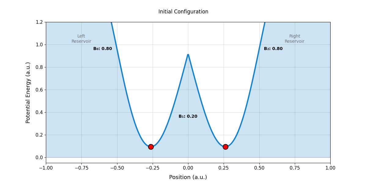
- Determines barrier sweep ranges:
- Outer barriers (B0, B2): From global turn-on voltage to mean transition voltage (decreasing tunnel coupling)
- Inner barrier (B1): From transition voltage to global turn-on voltage (increasing tunnel coupling)
- For each barrier configuration:
- Sets barrier voltages
- Runs
compute_peak_spacingto determine grid size - Runs
run_dqd_search_fixed_barriersto search for DQDs
- Early exits if
num_dqds_for_exitDQDs found at any configuration
Usage Notes:
- WARNING: Can be time-consuming! Default 5x5 grid = 25 barrier configurations
- Each configuration runs full peak spacing and grid search
- Middle barrier (B1) swept from transition to saturation ensures sufficient tunnel coupling for observable transition lines
- Higher tunnel coupling (B1 closer to transition voltage) typically yields more prominent transition lines
- Lower tunnel coupling (B1 closer to saturation voltage) may form bias triangles, harder for ML models to detect
- Results ordered by barrier sweep, find successful configurations with
[r for r in result['run_dqd_search'] if len(r['dqd_squares']) > 0]
Machine Learning Classifiers
DQD search uses several specialized ML models trained on quantum dot measurement data [1]. For detailed specifications and performance metrics, refer to the Models documentation:
- Coulomb Blockade Models: Used for fast screening (Stage 1) and peak spacing computation.
- Charge Stability Diagram Models: Used for detecting double quantum dot features in low-resolution (Stage 2) and high-resolution (Stage 3) scans.
All classifiers return a score indicating confidence. Higher scores indicate stronger feature detection. The hierarchical use of classifiers minimizes total measurement time by filtering out unpromising regions early.
Configuration Guide
Device Configuration
DQD search requires proper gate type annotations and sufficient plunger gates:
ML Model Setup
To use the machine learning classifiers, you must initialize the Conductor Quantum SDK using the setup_models_sdk routine. This routine authenticates with the platform and makes the models client available to the DQD search routines.
Add it to your configuration sequence before running DQD search:
Then ensure it runs before your search routines:
Routine Parameters
Key parameters to tune for your device:
Peak Spacing:
Trade-offs:
- Wider scale range: More likely to find peaks, but longer computation time
- More samples: Better statistics, but slower
- More trace points: Better resolution for peak detection, but slower per trace
Grid Search Resolution:
It is recommended to use the default resolutions as the machine learning models provided with Stanza are specifically designed and trained for these input sizes (128/16/48).
Changing these resolutions is discouraged as it may significantly degrade model performance. The default models expect these specific input dimensions. Only modify these parameters if you are supplying your own custom ML models trained on different resolutions.
Search Control:
Trade-offs:
- Larger max_samples: More thorough exploration, longer measurement time
- Higher num_dqds_for_exit: Find multiple DQD regions, takes longer
- include_diagonals=true: Denser exploration (8 neighbors instead of 4), may find nearby DQDs faster
Nested Routine Execution
Organize DQD discovery as a nested routine workflow:
Execute the entire workflow:
Advanced Usage
Visualizing DQD Results
Extract and visualize high-resolution charge stability diagrams:
Custom Barrier Configurations
Run DQD search with specific barrier voltages:
Best Practices
1. Always Complete Health Check First
DQD search requires voltage bounds and gate characterization:
2. Start with Fixed Barriers
Use run_dqd_search_fixed_barriers before full barrier sweep:
3. Use Appropriate Resolution
Balance measurement quality vs time:
- Quick exploration: 128/16/32 (current_trace/low_res/high_res)
- Standard quality: 128/16/48 (recommended starting point)
- Publication quality: 128/32/64 (slower but better CSDs)
4. Monitor Peak Spacing Results
Verify peak spacing is reasonable:
5. Set Reasonable Exit Conditions
num_dqds_for_exit=1 is often sufficient:
6. Validate DQD Discoveries
Visually inspect high-res CSDs:
7. Use Reproducible Seeds
Set seed parameter for reproducible random sweeps:
Troubleshooting
No Peak Spacings Found
Symptom: ValueError: No peak spacings found.
Causes:
- Health check not completed
- Voltage scale range too narrow
- Device not showing Coulomb blockade
- Barrier voltages not optimal
Solutions:
- Verify health check completed: check
ctx.resultsfor gate characterization - Increase
max_search_scaleto test larger voltage ranges (e.g., 0.3 V) - Increase
max_number_of_samplesfor more attempts per scale (e.g., 50) - Check device connectivity and current measurements
- Try manual barrier voltage adjustments for better tunnel coupling
No DQDs Found in Grid Search
Symptom: dqd_squares is empty after search completes
Causes:
- Barrier voltages don’t allow sufficient tunnel coupling
- Peak spacing incorrect
- Plunger voltage bounds too narrow
- Grid resolution too coarse
Solutions:
- Try
run_dqd_searchto sweep barrier voltages: - Increase
max_samplesto explore more grid squares - Verify plunger voltage bounds are adequate (check health check results)
- Increase
high_res_csd_pointsfor better resolution (e.g., 64 instead of 48) - Review logged low-score squares - may indicate near-misses
Grid Search Too Slow
Symptom: Search takes too long to complete
Causes:
- Resolution too high
- max_samples too large
- Grid too fine (peak spacing too small)
Solutions:
- Reduce resolution: use 128/16/32 instead of 128/16/48
- Reduce
max_samplesfor faster termination (e.g., 20% of grid) - Set
num_dqds_for_exit: 1to exit after first DQD - Use
include_diagonals: falsefor sparser exploration - If peak spacing is very small (
<30 mV), consider adjusting search scales
False Positive DQD Classifications
Symptom: High-res CSDs don’t show clear DQD features
Causes:
- ML classifier over-predicting
- Measurement artifacts or noise
- Insufficient resolution
Solutions:
- Review top candidates visually - plot high-res CSDs
- Check
total_scorevalues - higher scores (>2.0) more reliable - Increase
high_res_csd_pointsfor clearer features (e.g., 64) - Review Stage 1 and Stage 2 scores - all stages should agree
- Consider manual validation of top candidates
Voltages Out of Bounds
Symptom: Grid squares skipped or voltage errors during search
Causes:
- Grid extends beyond safe voltage bounds
- Gate characterization voltages incorrect
Solutions:
- Check leakage test results for safe voltage bounds
- Verify gate characterization completed successfully
- Algorithm automatically skips out-of-bounds squares - this is expected
- If too many squares skipped, adjust plunger voltage bounds in device config
Complete Example: DQD Discovery Workflow
Here’s a complete example from health check to DQD discovery:
References
[1] Moon, H., et al. Machine learning enables completely automatic tuning of a quantum device faster than human experts. Nat Commun 11, 4161 (2020). https://doi.org/10.1038/s41467-020-17835-9
[2] Zwolak, J. P., et al. Autotuning of double-dot devices in situ with machine learning. Phys. Rev. Applied 13, 034075 (2020). https://doi.org/10.1103/PhysRevApplied.13.034075
[3] van der Wiel, W. G., et al. Electron transport through double quantum dots. Rev. Mod. Phys. 75, 1 (2002). https://doi.org/10.1103/RevModPhys.75.1